
(Editor’s note: 8th & Walton offers Retail Link classes for new analysts and seasoned suppliers. Before taking your first class with us, it’s best to familiarize yourself with these basic Excel functions to make the data work for you.)
Walmart suppliers get their weekly sales data from Retail Link. What new suppliers may not realize at first is Retail Link only provides the raw data. For proper analysis and forecasting, the information needs to be downloaded into an Excel spreadsheet.
Beginning Retail Link analysts are sometimes surprised at how knowledgeable they must be at Excel. You do not have to be an expert, but mastering a few functions will make the weekly reporting and formatting much easier!
Basic Excel Functions for Analysts
The following Excel functions are a must for the Retail Link analyst. Click on a function to jump to a full description:
1. Copy and Paste
If you are new to Excel, copy and paste work as they do in other applications. You also have a variety of ways to copy data from one area and paste it in another.
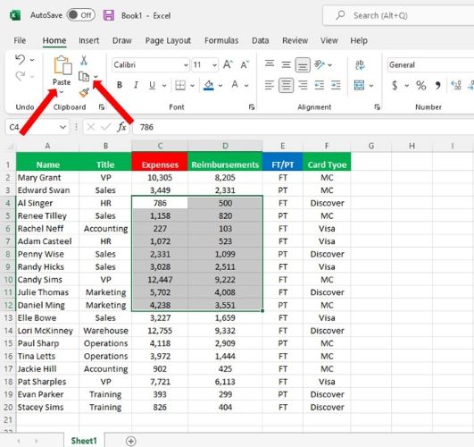
After selecting the row, column, or cell(s) you wish to copy, your first option is to use the copy and paste buttons located in the top ribbon as shown below:
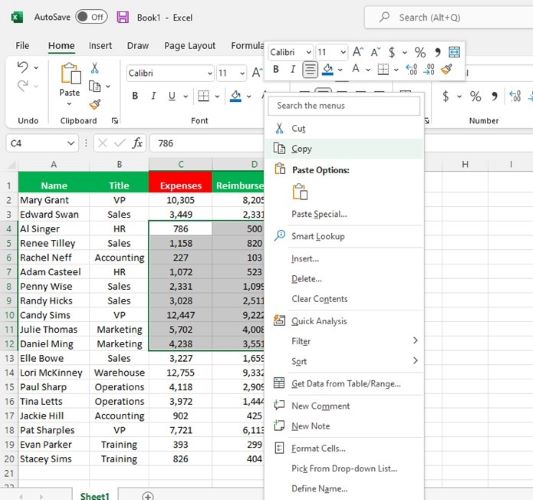
The second option is to right-click on your mouse or touchpad to bring up the edit menu. Copy and paste can be found at the top as shown below:
For those who prefer editing options on their keyboard, simply hit CTRL and C to copy cells. To paste the data in its new location, hit CTRL and V.
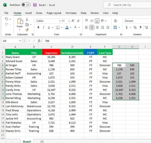
Copy the selected cells in whichever method you prefer. When you’re ready to paste, click on the cell where you want the copied data to begin. The data will fill out the new destination cells as it was from where it was copied as seen below:
2. Filters
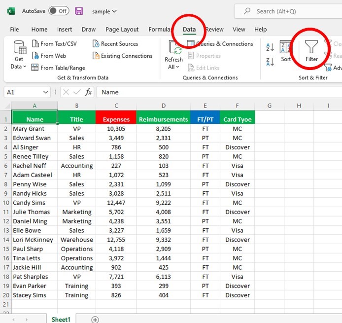
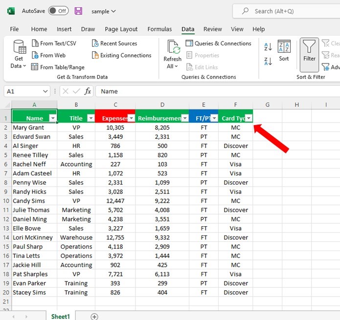
Applying a filter to columns in an Excel spreadsheet allows you to view data quickly by a selected criteria. For example, in the spreadsheet below, we want to only see employees who paid for their company expenses using a Visa card. The first action is to click on the Data tab and select Filter.
After clicking Filter, the drop-down buttons will be added to the top of each column as seen below:
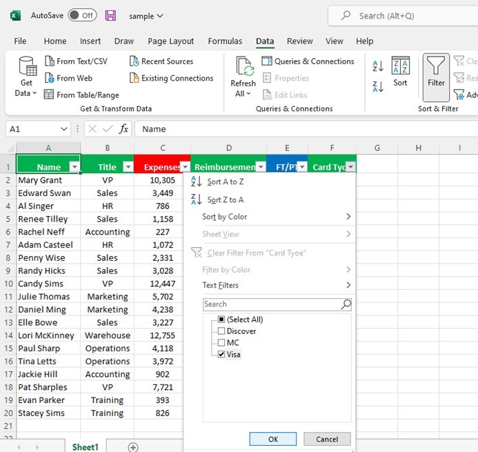
To see only the employees who paid their expenses with a Visa card, we would click on the drop-down button in the Card Type column. When the menu pops up, we then deselect all criteria except Visa and click OK.
The data has now filtered to only show employees paying with a Visa card.
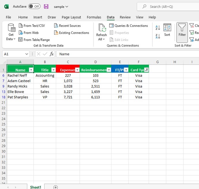
When using a filter, it is possible to filter within a filter. For example, you can first filter by all employees who paid their expenses with a Visa card, then filter that group by employees in Sales.
3. Sorting Columns
Sorting columns in your spreadsheet allows you to see and analyze your data better. You can organize and find the data that you need in the order you prefer. This function allows you to quickly arrange your spreadsheet by column alphabetically or numerically in ascending or descending order.
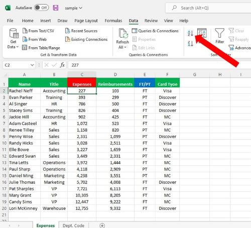
In our expense report example, let’s assume we want to view the report from the person who spent the least amount of money up to the person who spent the most. To arrange the spreadsheet in ascending order by the Expenses column, we click on the Data tab and select the first cell of the column. We then locate the Data Sort section of the ribbon as seen below:
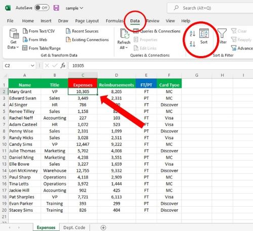
Next, we click on the A to Z option. This arranges the Expenses column in ascending numerical order. The rest of the spreadsheet data will change to align accordingly.
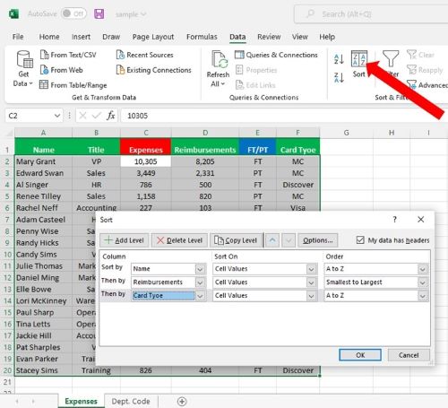
The Sort function also allows you to sort multiple columns in multiple options. Simply click on the larger Sort Columns option to bring up the menu. Clicking the Add Level option allows you to add more selections to sort multiple columns according to your data needs.
4. Conditional Formatting
Conditional formatting allows the analyst to highlight certain values or make specific cells easy to locate. This function changes the text or background fill of cells based on rules you create. Analysts use conditional formatting to highlight cells that contain values which meet a given criteria.
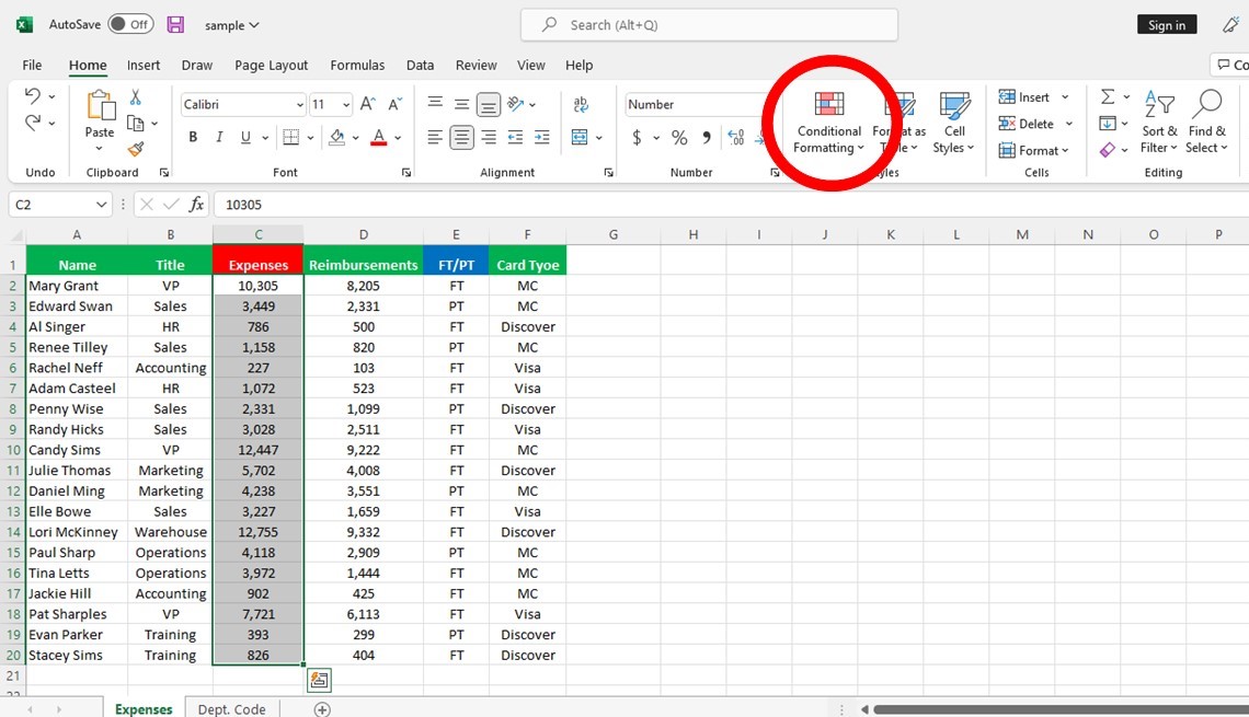
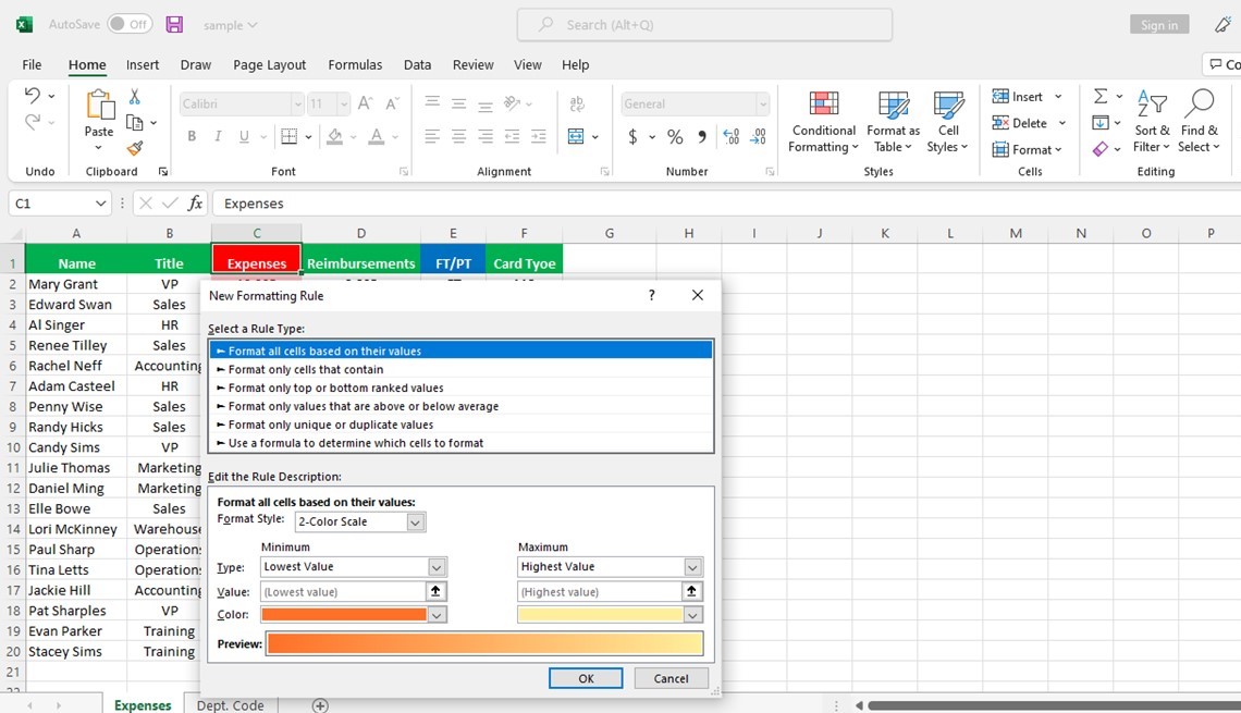
In our expense report example, we’ll set a very quick and basic conditional formatting rule. If we want to quickly identify all expenses over $4,000, we first highlight all cells under Expenses and click on Conditional Formatting.
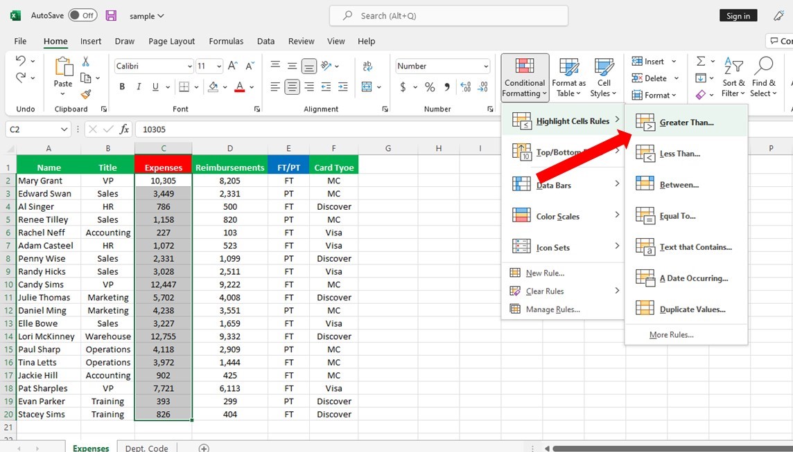
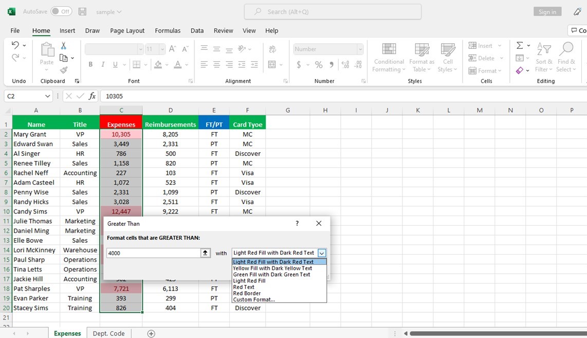
Under the Conditional Formatting button, we select Highlight Cell Rules and Greater Than:
When the Greater Than menu pops up, fill in the number 4000 and select a color scheme. For this example, we’ll select all expenses over 4000 dollars to appear with red text on a red cell background.
Each cell containing a value over 4000 will now adapt to the new rule of conditional formatting. If you were to set this rule on blank cells, the rule would apply after the value was entered.
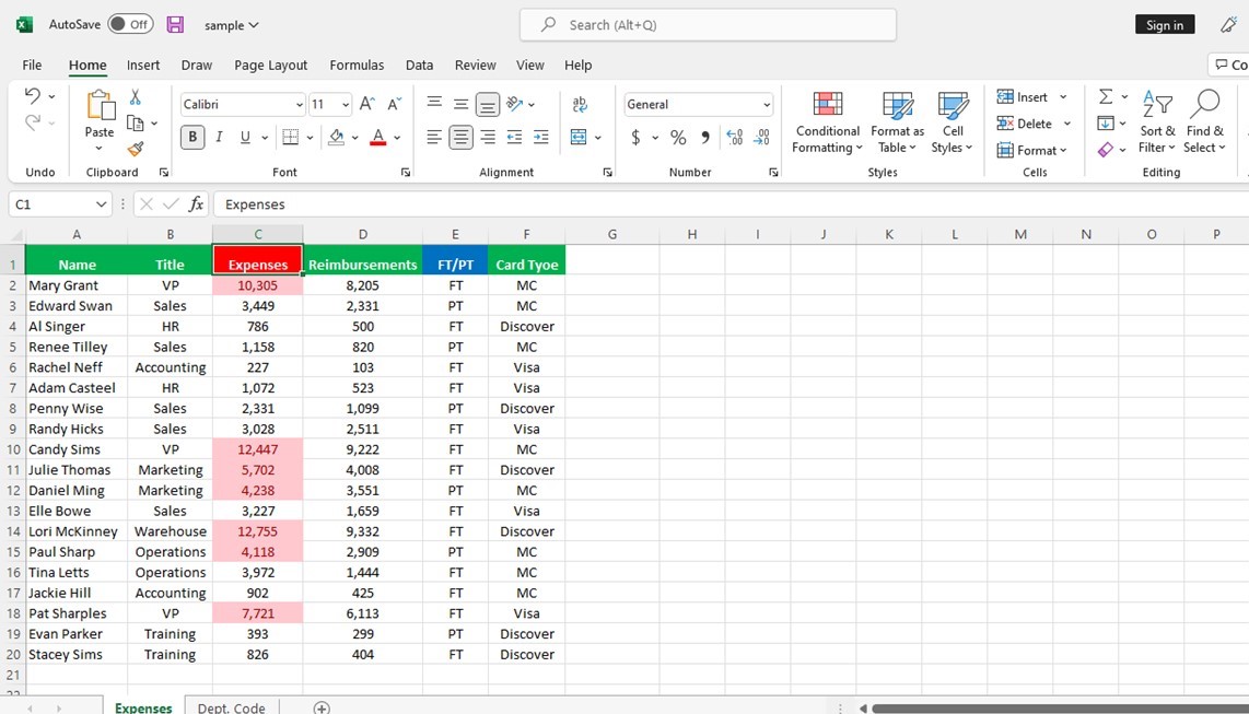
This is a very basic example of how to use Conditional Formatting for data analysis. The function also allows you to set your own formatting rules based on the data, ranges, conditions, and identifiers you specify. Play with Conditional Formatting in your spreadsheets to find what schemes work best for your analysis.
5. Countif
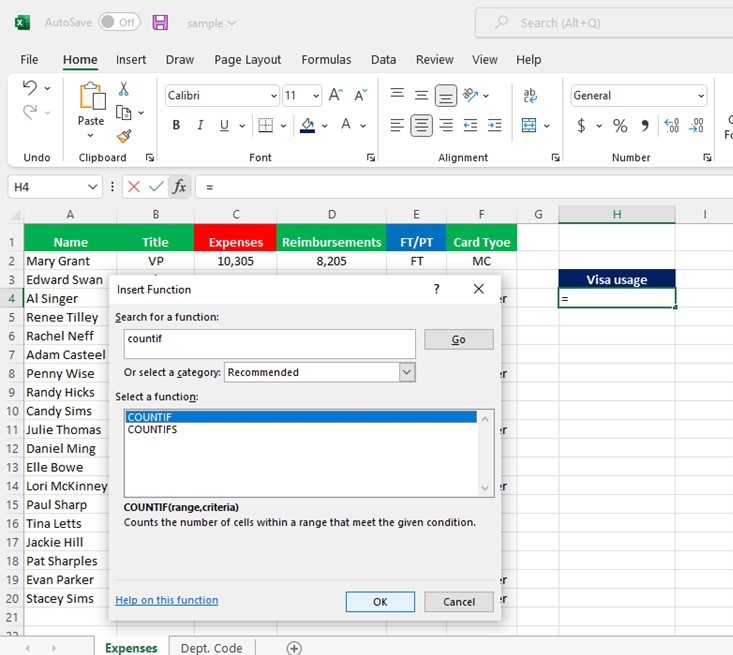
The Countif function allows you to quickly total the number of cells that meet a specific condition or criteria.
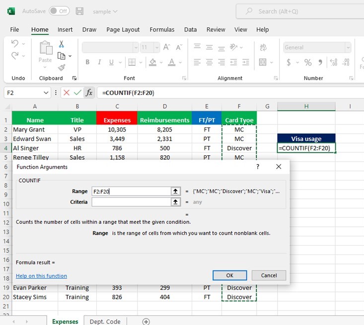
In our expense report example, we can find the total number of times a Visa card was used by brining back a count of how many times the word “Visa” appears in the Card Type column. Begin by selecting a destination cell (we have selected cell H4 below), click the fx button, and select Countif.
Next, select the range of data you wish to be scanned. In this case, we select the Card Type column.
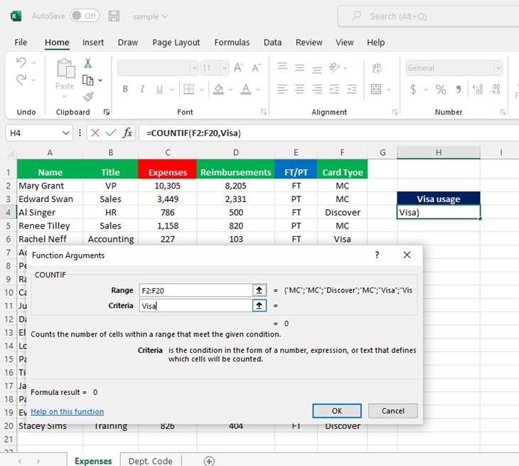
Finally, select the criteria you want to count. Type the word Visa, or select a cell with the word Visa. Click OK.
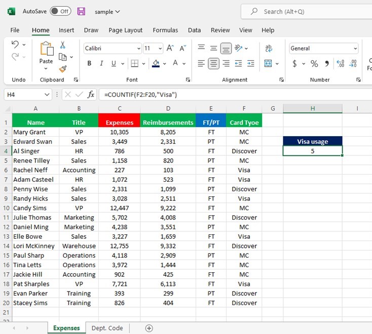
The formula now totals the number of times the word Visa appears in the column.
6. Sumif
The Sumif function allows you to quickly total values of cells that meet specific condition or criteria.
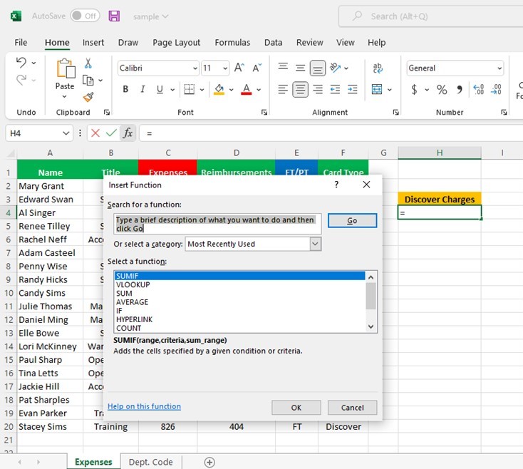
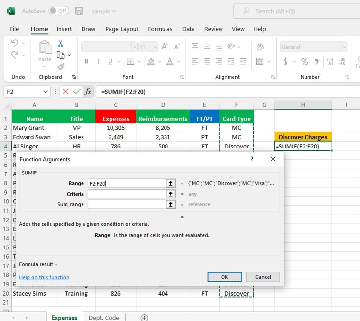
In our expense report example, we can find the total of how much money was spent using a Discover card. We first select a cell (in this case cell H4 below) and click the fx button to select the Sumif function:
Next we select the range containing the criteria we wish to total. Because we want to look for totals on Discover cards only, we select the values in the F column.
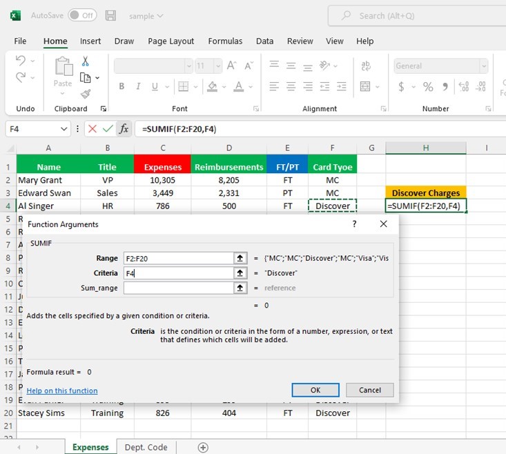
We then select the specific criteria in the range for which we are looking for totals. Because we only want Discover, we can click on cell F4.
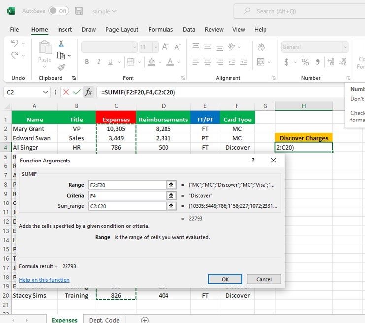
Finally we select the Sum Range. This is the column where the values are located that we want to total. In this example we want the expenses from Discover cards, so we highlight all of the values in column C. We then click OK.
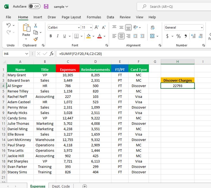
Applying the Sumif function now brings back the total for all expenses assigned to Discover cards.
7. Vlookup
The Vlookup function (“vertical lookup”) allows you to pull data from one spreadsheet into another by using a common value between the two.
In the expense report example we’ve been using, we’ve added a second spreadsheet: department codes. We want to add a department code column to our original spreadsheet, but do not want to manually copy and paste each corresponding code to the department on our original spreadsheet. The Vlookup function will search and find the right number.
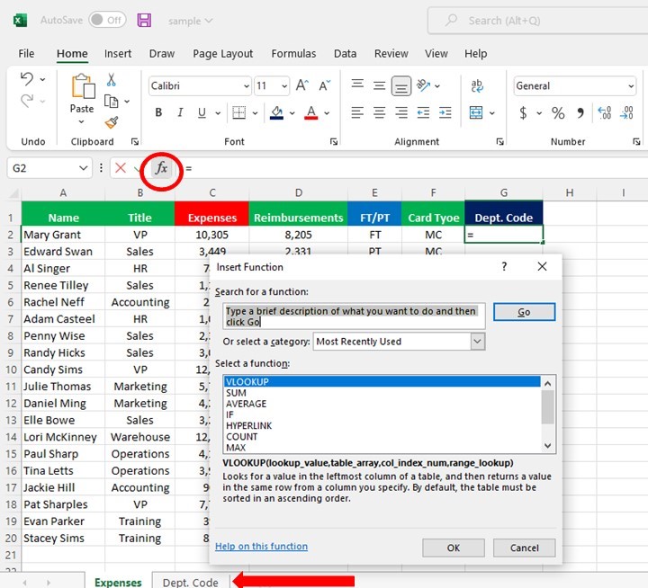
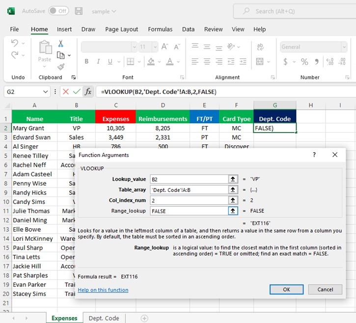
To begin, select the first cell where you want the new data to go. In the function bar, type “=VLOOKUP” or click the “insert function” button and select VLOOKUP. Click OK to begin.
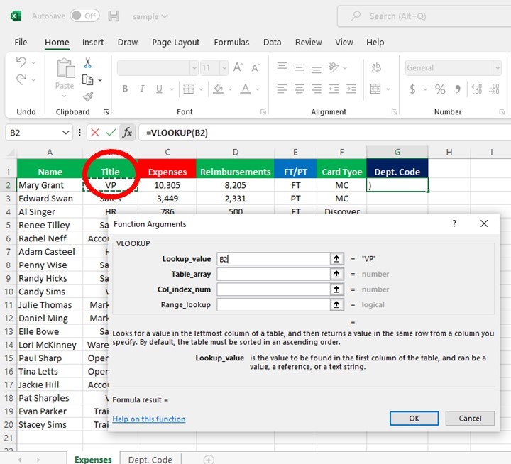
When the next menu pops up, you must provide four pieces on information. First, enter the Lookup Value by clicking on the common value between the two spreadsheets. In this case, the Lookup Value is the information in the Title column, so we click on cell B2.
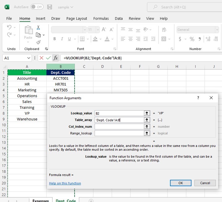
Second, we select the Table Array. We do this by going to the spreadsheet where we wish to retrieve information (the Dept. Codes tab) and highlighting the two columns.
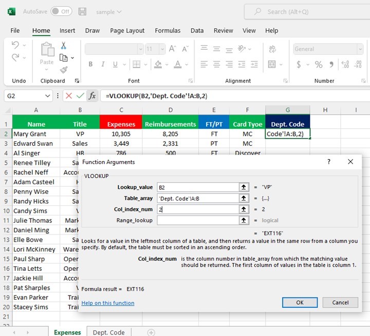
Third, we must enter the Column Index Number. In this case, the column on the Dept. Code spreadsheet which holds the information we want to retrieve is second from the column that has the common data of our Expenses spreadsheet. Therefore, we enter the value 2.
Finally, we enter the Range Lookup. Enter the word FALSE. This tells the Vlookup that you want an exact match to the value you are looking up. Click OK.
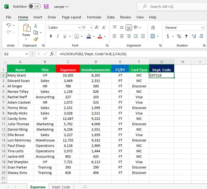
Your selected cell should now be populated with the corresponding value on the sheet you are pulling from.
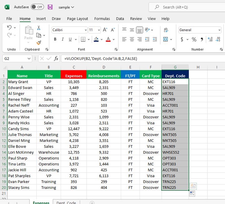
You do not have to perform this function for each corresponding row in the column. You can simply drag the formula down the column and each row will populate with the data from the spreadsheet from which you are pulling.
Conclusion
Understanding these basic Excel functions is key to better data organization for Retail Link analysts. If you have questions about your weekly reporting, Retail Link, or how use the data to make your business more profitable, request a free consultation with one of our Walmart advisors.
Complete the form below to schedule your free consultation.